Rudolf Riedi: Research Synopsis

Multiscale Statistics for Evolving Complex Systems

An easy-read on multiscale mehodologies

The relevance of multiscale modeling

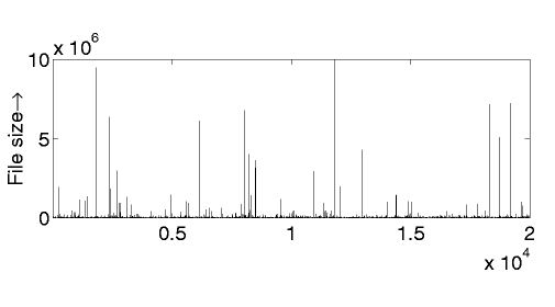
It has for long been realized that efficient and accurate modeling of various real world phenomena needs to incorporate the fact that observations made on different scales each carry essential information. In most simple terms, representing data on large scales by its mean is often useful (such as as `average income' or an 'average number of clients per day') but can be inappropriate. Examples include the arrival of clients in a waiting queues (Fig. 1), stock returns and indices, local connectivity in a large scale heterogeneous ad hoc network, geophysical well-data, measured velocity in fully developed turbulence and many more.

Resolution	Real WAN Traffic	MWM Multiplicative model	fGn Additive model
6msec		$[Multifractal model at 6 msec]$
24 msec		$[Multifractal model at 24 msec]$

Fig 1: The multiplicative Multifractal wavelet model outperforms the additive Gaussian model

Classical models of time series such as Poisson and Markov processes rely heavily on the assumption of independence, or at least weak dependence. So do classical limit theorems such as the Law of Large Numbers which states that at large scales a Poisson process can safely be approximated by its mean arrival rate. However, in real world situations one is confronted with data traces which are `spiky' and `bursty' even at large scales. Such a behavior is caused by strong dependence in the data: large values tend to come in clusters, and clusters of clusters, or by infinite variance effects. This is as true for the classical data of the River Nile as for modern high speed communication networks and has obvious and far-reaching consequences ranging from reservoir and buffer design to bandwidth allocation to name but a few.

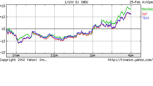
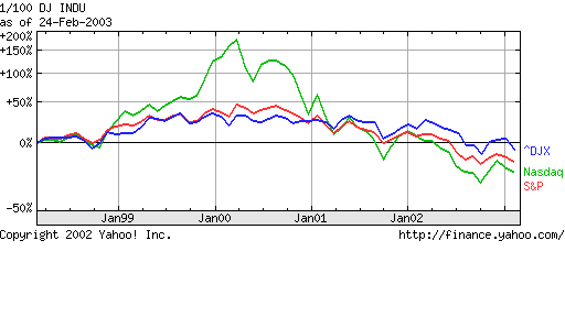
Fig 2: Nasdaq, S&P500 and Dow Jones indices show rich detail at fine and coarse time granularity

Fractal Models

Aimed at modeling at multiple scales, fractional Brownian motion (fBm) is able to capture and incorporate long range dependence (LRD) at least in terms of second order correlations. In this attractive fractal model, LRD is directly coupled to a rescaling property which makes fBm look `statistically identical' on all scales. Being a Gaussian process fBm is a natural candidate for an approximation of LRD-traces, at least at large scales due to the Central Limit Theorem (CLT) which states roughly that sums of random variables (ie. highly aggregated or large-scale data) tend to the Normal distribution.

Self-similarity: Statistical Scaling of FBM

Well-log

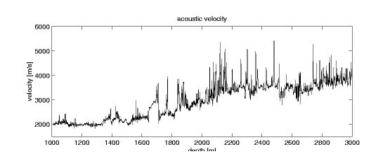
Web requests

Fig 3: The scaling of the Gaussian FBM-process can capture Long Range Dependence.
Yet, it may provide a poor approximation to certain real world data.

Multifractal Models

Like fractal models, multifractals are inherently multiscale objects with strong rescaling properties, but with the essential difference of being built on multiplicative schemes. Naturally, they are highly non-Gaussian and are ruled by different limiting laws than the additive CLT, more precisely by martingale theorems. Moreover, multifractals exhibit exactly that `spiky' and `bursty' appearance which we encounter now in many real world situations such as Internet traffic loads, web file requests, data of interest in turbulence at high Reynolds numbers and in Geophysics, to name but a few.

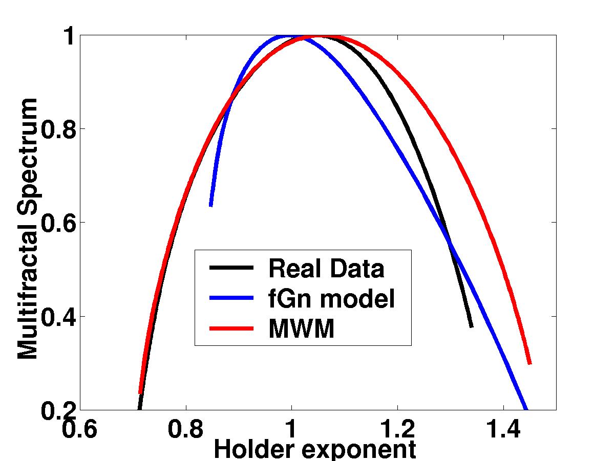
Multifractal spectrum

The LRD built into fractal models helps address strong correlations and high variability, especially on large scales or aggregation levels. Bursts, however, are much better understood in terms of a local scaling analysis which is designed to capture not only an overall behavior but rather also rare events such as bursts. This is exactly what the multifractal spectrum f(a) provides in terms of a large deviation principle: given the strength of a burst measured with the exponent a the value f(a) indicates how frequently this strength a will be encountered. The larger f(a) the more often one will see a.

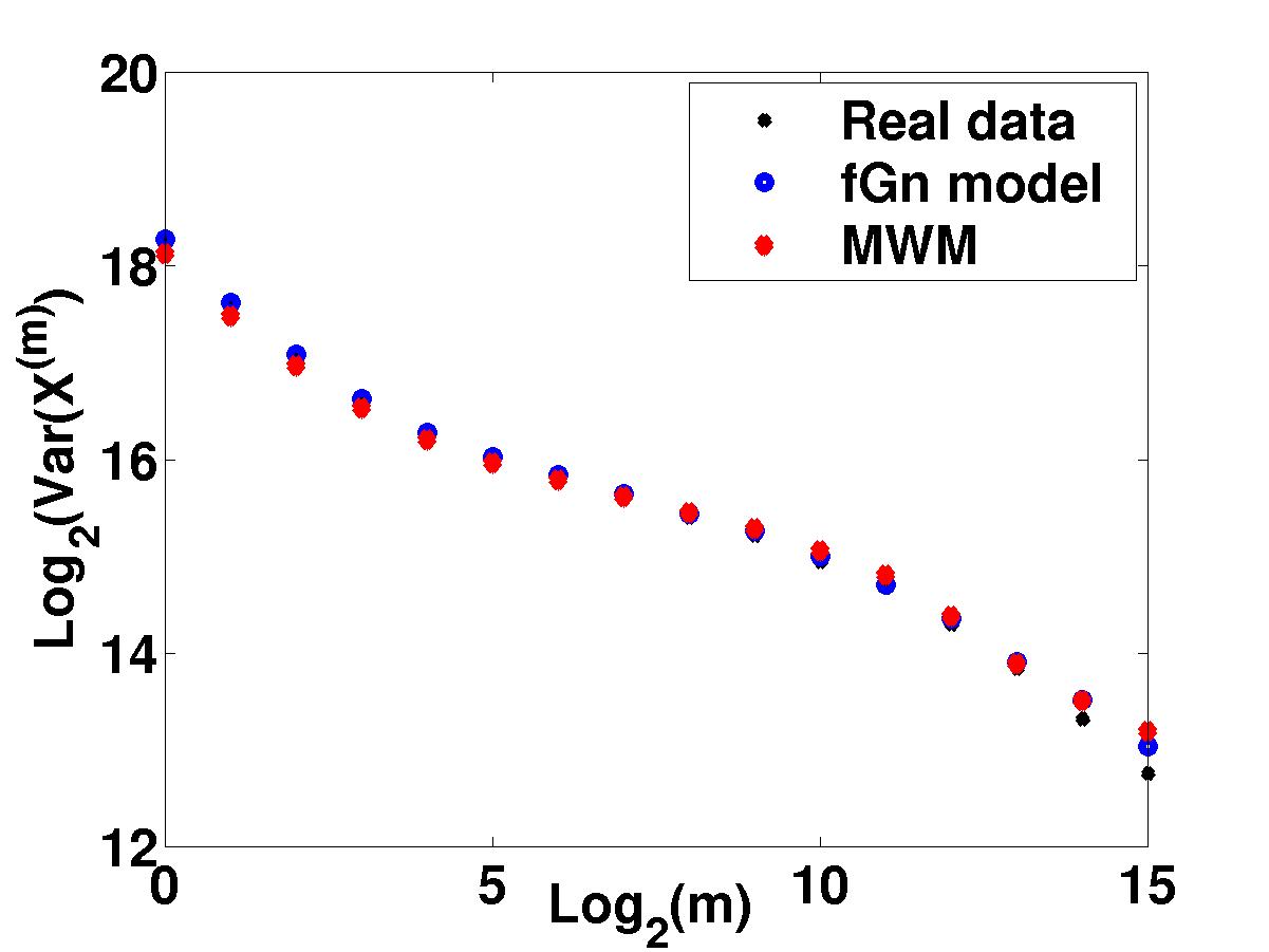
Effectiveness and accuracy of multiplicative, multifractal models

We make the case for multifractal modeling with the example of network traffic modeling in Fig 4.

Variance time plots indicate that both the MWM and the fGn exactly match of the second-order correlation structure of the Bellcore data of Fig 1.
Yet, there is a clear difference in the quality of approximation of the two models which we address now.

The Multifractal spectrum measures the "burstiness" of a time trace through the scaling of its higher-order moments. Note the close match between the spectra of the MWM and Bellcore data, particularly in the left half of the curves. This is a quantitative explanation for the close visual match we see above. In contrast, the fGn match is poor. The MWM comes with its own toolbox of powerful multifractal analysis techniques for characterizing traffic burstiness and long-range-dependence.

More important than either the visual or multifractal spectrum match is the fact that the MWM synthesized data has nearly the same queuing behavior as the real data, again in contrast to the fGn model. Here we plot the queue overflow probability as a function of queue size.
Exploiting the tree-structure of the MWM we have developed an
analytical formula for the queuing behavior of MWM traffic, which will be vital for online traffic characterization and performance prediction, as well as an
adaptive algorithm to infer competing cross traffic along a path through the internet.

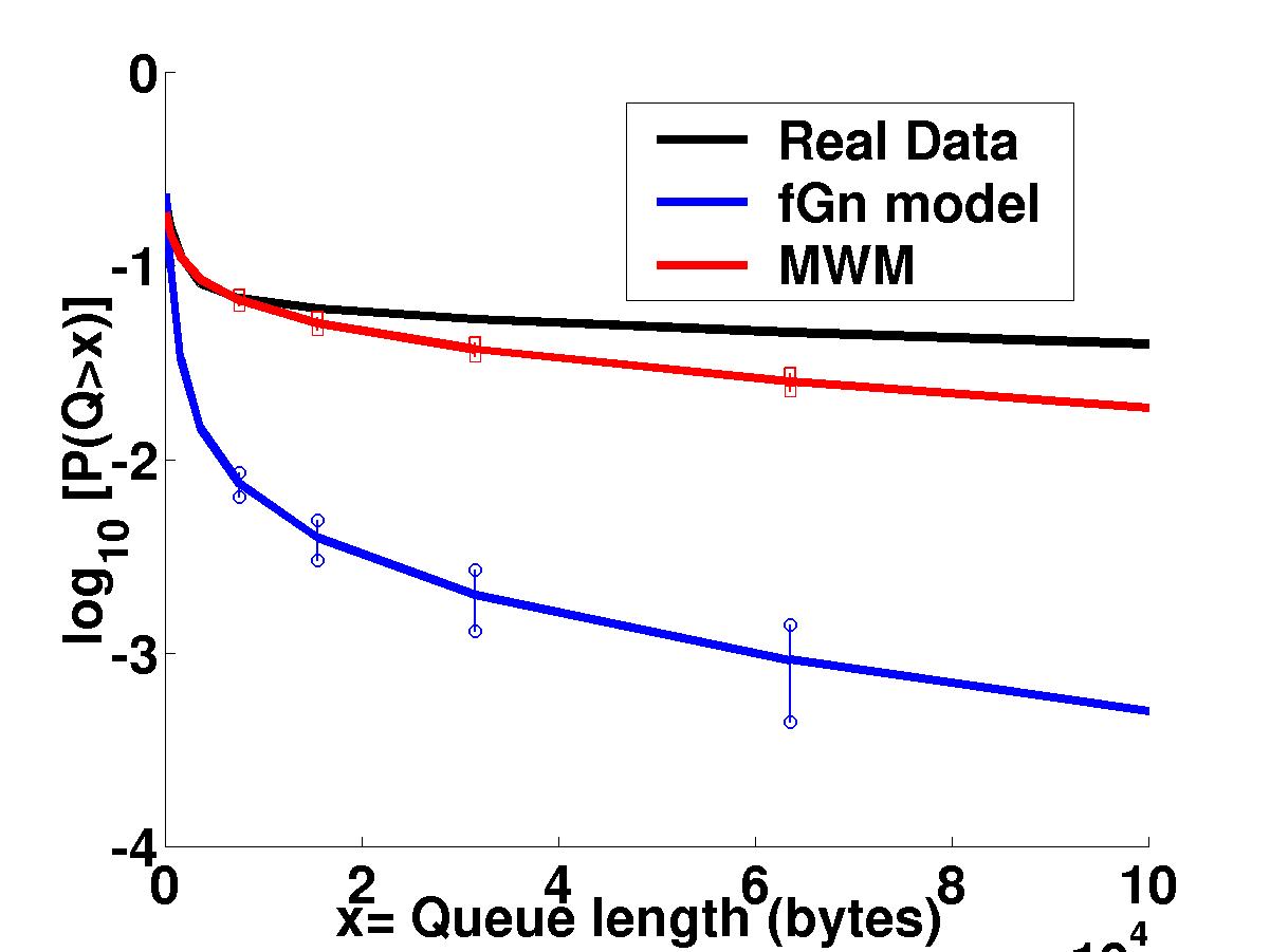Fig 4: Explaining the superiority of multiplicative traffic modeling.

Variance time plots indicate that both the MWM and the fGn exactly match of the second-order correlation structure of the Bellcore data of Fig 1. Yet, there is a clear difference in the quality of approximation of the two models which we address now.
The Multifractal spectrum measures the "burstiness" of a time trace through the scaling of its higher-order moments. Note the close match between the spectra of the MWM and Bellcore data, particularly in the left half of the curves. This is a quantitative explanation for the close visual match we see above. In contrast, the fGn match is poor. The MWM comes with its own toolbox of powerful multifractal analysis techniques for characterizing traffic burstiness and long-range-dependence.
More important than either the visual or multifractal spectrum match is the fact that the MWM synthesized data has nearly the same queuing behavior as the real data, again in contrast to the fGn model. Here we plot the queue overflow probability as a function of queue size. Exploiting the tree-structure of the MWM we have developed an analytical formula for the queuing behavior of MWM traffic, which will be vital for online traffic characterization and performance prediction, as well as an adaptive algorithm to infer competing cross traffic along a path through the internet.