Overview

XploRe -- the interactive statistical computing environment -- provides a professional set of computational tools for statistical analysis. The environment XploRe is a powerful tool of computational statistics for data analysis, research and teaching which comprises a full, high-level object oriented programming language.

XploRe has a client/server architecture which yields an enormous amount of networking facilities in methods and data. XploRe can be installed on an Inter- or Intranet server. Due to the revolutionary Java Interface, it can be accessed by any client. This pathbreaking innovation in the world of software engineering in combination with the highly interactive graphics turns XploRe into one of the most powerful and flexible tools in computational statistics.

Moreover, XploRe supports the dynamic linking of procedures written in any one of the common programming languages (like C++, Fortran or Pascal). If you have written your own procedures and are looking for a powerful visualization tool, XploRe is just what you need.

XploRe is equipped with a lot of statistical functions. The user has the possibilities to customize XploRe to his specific needs. Moreover, XploRe provides possibilities for any kind of graphical representation of data structures. XploRe is able to create a great variety of multiple graphical objects.

Variables can be collected in structures, so that it is possible to hold common information of a data set in a single data object. Thus all the features of a high-level object oriented language like recursion, local variables, loops, and conditional execution are available.

XploRe provides an interactive help system in the standard UNIX or Windows format which not only allows the direct access of help at any instant but also supports ``learning statistics by doing statistics''.

XploRe can be used as a basis for research, courses in statistical model building, computational statistics and computeraided teaching. The user interface and the help system have been psychologically tested and optimized. It is successfully used in large courses on applied multivariate statistics, computer-aided statistics and econometrics. The interactive help system gives you the possibilities to access - or even write - tutorials about the use of XploRe and the implemented statistical methods. Overall, XploRe is an ideal tool for the development and use of Teachware.

XploRe is infinitely flexible. You can add your own procedures or libraries to work out a particular computing environment customized to your specific needs. Thus, the environment XploRe can be optimally shaped by the developer himself. Thus, XploRe is a toolkit for software development.

XploRe already comprises a lot of statistical methods, that can be used interactively. These methods are stored in different libraries consisiting of several macros that are provided to your convenience. To keep the program as slim and efficient as possible, these libraries are loaded into XploRe whenever they are needed. These libraries are subsumed to different modules. This mirrors the manifoldness of statistical working ranges covered by XploRe.

Networking facilities for Methods & Data

The help system is available in HTML and can be easily read with a common WWW browser like Netscape, MS Internet Explorer, etc. Furthermore, the newly developed Java interface ensures that, installed on an Internet/Intranet server, XploRe clients run on every platform that supports Java. Thus, all XploRe features are online available.

This technology ensures, that a complete XploRe session can be opened just with a Java capable WWW browser. Moreover, such a browser is not necessary. With a Java virtual machine you are able to access all the features, that are available in a local installation.

The Java applets will generate a full graphical user interface, where local generation, interactive changing and all the other graphical features are possible without having access to the server.

You can access XploRe from anywhere in the world and you do not need much capacity for your calculations. Basic operations are executed on the server, whereas all the fine tuning is done on your client.

Moreover, XploRe procedures or even libraries can be called from a foreign host and are executed by the server before the result is given back to the Java client. This keeps the amount of data transmission low and reduces transaction time and costs.

To round off the networking facilities, XploRe is equiped with the possibility to execute remote procedure calls (RPC). Data is transported to other software, manipulated in the according way and reimported to XploRe.

Interactive Graphics

In XploRe, graphical objects can be interactively manipulated in any way you can imagine. They can be scaled, rotated, linked, brushed and changed in thousand other ways. For example, you can rotate a plot just by clicking on it and moving around the mouse pointer or pressing the arrow keys.

You can change the labels of either axis or endow the plot with a self chosen title. The complete outlook of the data can be changed. Points can be plotted as circles, stars, grids and any other sign you could have in mind. In the same way, lines can be designed solid, dashed and so on.

The plots can be saved and printed from the screen as PostScript files to be later used in any kind of presentations, scientific working papers etc. - or maybe you would like to decorate your Internet homepage or a birthday card with it.

As all these graphical features are present in the local version, you can access them in the same manner with the Java Interface on every machine that supports a Java virtual machine or by simply using a web browser.

Matrix operations

XploRe comes with the standard operations for an easy handling of arrays. It contains functions for matrix calculations like multiplication, transposition, matrix inverse, determinant, calculation of eigenvalues and eigenvectors, complex algebraic calculations and many other. You can partition matrices or stack vectors. The matrix syntax is natural and easy to handle. The possibilities of matrix handling in XploRe are almost infinite.

Statistical functions

Additional to the mathematical functions, XploRe contains all the useful basic statistical functions. For example, functions for the computations of mean-vectors, (co-)variance-matrices as well as probability distribution functions or corresponding cumulative distribution functions are present.

Smoothing routines

One of the strengths of XploRe is, without any doubt, its competence in semi- and non-parametric modelling. It has been equiped with smoothing routines like Kernel smoothing, running mean, spline regression, monotone regression, locally weighted regression (LOWESS), isotonic regression, k-nearest neighbour, wavelets and any other kind of functions, that are used in nonparametric statistics.

2-dimensional graphics

For the standard plotting of 2-dimensional data, XploRe comprises allmost any known form of data presentation like scatterplots and scatterplot matrices, boxplots, overlaying of different plots as well as graphical handling like rotating, scaling, zooming and so on. You have interactive graphical control of line styles, labels, colors, title, brushing and all the features needed for an inspiring visualization of your data are provided by XploRe.

3-dimensional graphics

Additional to the common handling of 2-dimensional data, 3-dimensional data treatments like rotation, interactive graphical control, colors, interaction with mouse or hotkeys, changing the view on surfaces, take place in the same way.

Multiple graphics in one display

Each graphical display can be divided into different plot areas with different graphical styles (e.g. two 3-dimensional plots, one 2-dimensional plot and a text area with descriptive values). Any plot area can be manipulated in an individual way, like e.g. linking and brushing. You have one window with as many different graphical representations as you like and all masking facilities are available for each plot in each display.

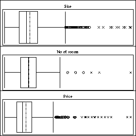
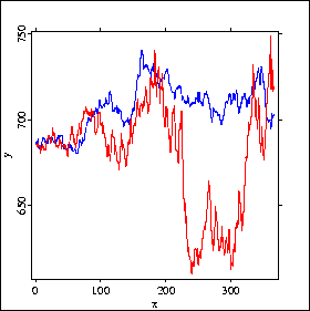
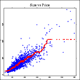
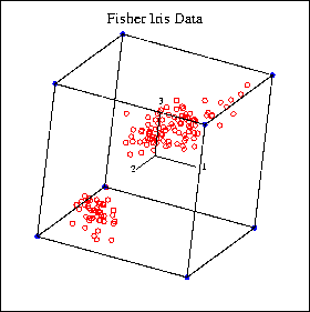
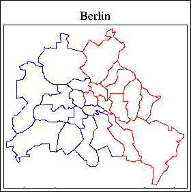
Examples for graphical representations in XploRe

The Help System

XploRe is fully documented in HTML. The help system can be accessed with any common WWW browser. That makes it easy to change between different help themes just by choosing the corresponding links.

The help system takes advantage of a new technology. Pages in your browser contain different - stationary and non-stationary - frames: the overview and the main keywords are allways present.

The explanation of the XploRe working environment is context-sensitive: an image is displayed, a click on the area information is needed about and the appropriate information is displayed. This way, XploRe can be ``explored'' by using the help system.

XploRe is equipped with a local helpfile system corresponding to the standard UNIX or Windows format. In the presence of a client-server installation, due to the HTML-format, it is not necessary to install it locally. It can easily be accessed with your web-browser.

Programming Examples

Furthermore, the help system contains a load of programming examples which are available with the underlying XploRe code. You can copy them for adapting several programming techniques and having a valuable reference for programming. They can easily be modified to customize XploRe to your actually needed purposes.

Short Help for Functions

For any function that is available in XploRe you have the possibility to access a short help. You can choose a function interactively from the working environment and the corresponding short help is displayed on the screen.

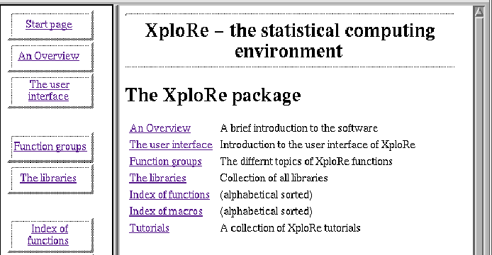
The help system

Interactive Learning with the HTML-Documentation

Two features of XploRe lead to its suitability as a teachware tool. The HTML written help system with a complete documentation of the XploRe package. On the other hand, there are libraries like the library Teaching Wavelets, which interactively guide you through a XploRe course. You are invited to carry out operations and check the results in the corresponding HTML documentation immediately.

The Tutorials

Additional to the online documentation of the XploRe commands, there exists a number of ``Tutorials'' where the use of XploRe can be learned. Moreover, the application of statistical methods is taught interactively. The tutorials provide a teaching tool which guides the user interactively through the application of XploRe and the implemented statistical methods. That makes learning statistical methods very easy and comfortable and overall a lot of fun. Inter alia, tutorials exist for the following themes:

• Graphics in XploRe
• Generalized Linear Models (GLM)
• Generalized Partial Linear Models (GPLM)
• Wavelets
• Neural Networks
• Finance
• Errors in Variables
• Smoothing Techniques

Teachware

All in all, XploRe is a complete teachware system. Teachware comprises a set of computer software tools for computer-aided interactive teaching of certain knowledge elements. The construction of teachware for statistical knowledge is a rather young field since it is supported by data structures and graphical interaction possibilities.

Next to the tutorials, XploRe contains libraries that provide such teachware. As an example, there is the library ``twave'' which interactively teaches the use of wavelet techniques. Moreover, even the development of commercial teachware as well as teaching of self-developped software is possible.

The XploRe Language

XploRe offers a full flegded programming language. It can be used to extend the number of statistical algorithms by user written procedures. Through a library concept these new algorithms appear to the user like the regular XploRe commands.

These macros can be collected in libraries which can be embedded into the already present libraries. This open system strategy ensures and offers the use of XploRe in different research and application fields.

The XploRe language is intuitive and even the inexperienced user can without major difficulties reproduce the examples presented in the help system and use them as a basis for further investigation. The highly interactive graphics makes it possible to write teachware which can be used in research, lectures and teaching as well as for commercial purposes.

The XploRe system can be used as an efficient computing environment for a large number of statistical tasks. The computing tasks range from basic data and matrix manipulations to interactive customizing of graphs and to dynamic fitting of high dimensional statistical models.

Generating Help Files in XploRe

Usually, programming of a help system needs the same time as software development itself. This expenditure must no longer be wasted. XploRe is generating the help file for you. This is done for any user-written macro by an implemented function called ``Make Help''. The self-generated helpfile will be in the HTML format. No more adjusting work is necessary.

The Editor

As a rounding off, XploRe is equiped with an easy to handle editor that supports mouse operations like drag & drop. This turns XploRe into a very comfortable computing environment. For example, a button for the direct execution of your macro is present as well as one for the generation of the corresponding help file.

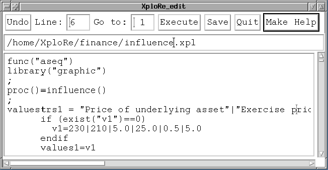
The XploRe Editor

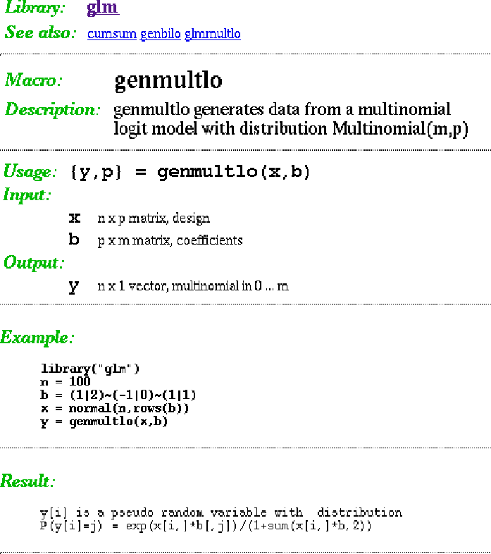
A self-generated help file

As a completion of the basic features of XploRe, the basic version is endowed with four basic libraries. They provide easy functions which provide a maximum of comfort for all statistical tasks. These are

• Basic Procedures (``xplore'')
• Graphics Library (``graphic'')
• Complex Numbers (``complex'')
• Teaching Wavelets (``twave'')

The libraries contain the basic statistical methods for estimation and visualization of data. They round up XploRe to a comprehensive statistical package. As a special bonus, the basic module contains the Teaching Wavelets library (``twave'').

The Basic Procedures library (``xplore'')

The library (``xplore'') consists of basic macros for statistical computations. It gives XploRe all the capabilities of a powerful programming language. Simple canonical elements of matrix calculation like diagonal or unitary matrices are present as well as basic mathematical and statistical functions for computing with matrices (like Kronecker-products, calculation of singular value decompositions and other advanced tools of multidimensional computation). Moreover, it comprises all basic statistical procedures as e.g. linear regression (OLS, GLS), contingency table analysis, factor analysis or principal component analysis. It further provides routines for descriptive statisics and handling of missing values.

The Graphics library (``graphic'')

The library (``graphic'') is a powerful tool for the visualization of data. It contains macros for plotting data in any way you could imagine. For example, it offers histograms, boxplots, 2- and 3-dimensional contour and surface plots, parallel coordinate plots, dotplots, Andrews curves plots, sunflower plots and many more. The library also provides programming tools for data transformation, rotation, etc. Furthermore, basic estimation procedures are already implemented. As an example you can interactively generate a linear regression plane (or line) to be added to your data plot.

The Complex Numbers library (``complex'')

The library (``complex'') comprises macros for standard operations and calculations with complex arrays like complex multiplication and so on. Moreover, useful functions as e.g. hyperbolic functions, matrix inversion and sorting are defined in this library.

Bonus: The Teaching Wavelets library (``twave'')

The library (``twave'') is an interactive teaching program to get familiar with the use of wavelets. You can interactively force approximation, soft thresholding, hard thresholding, data compression, image denoising, compute frequency shifts as well as the translation invariant or generate father and mother wavelets. The result can be checked immediately in the wavelet tutorial. That makes learning wavelet methods very easy, comfortable and overall a lot of fun.

The Time Series library (``times'')

Any variable that varies over time can be viewed as a time series. This general statement implies that analysis of time series takes place in almost any research field that deals with statistics. Time series play a central role in the investigation of interest rates, price fluctuations or other macroeconomic variables like GNP, exchange rates, inflation rates, and so on.

In time series analysis, one is mainly interested in the dependency of one variable or system of variables of its predecessors. The aim is to estimate a functional coherence between them and - what is of even more interest in most cases - construct a proper forecast.

In the last decades, there has been growing interest in the behaviour of non-linear time series such as the class of autoregressive conditional heteroscedastic (ARCH) models or generalized ARCH models (GARCH). These models occur mainly in the context of financial time series and play a central role in the modelling of volatility processes.

Details

The library (``times'') contains simulation, estimation and forecasting procedures for the standard (e.g. ARMA or VARMA models) as for recently developed models of the ARCH, GARCH, TGARCH or related types. For example, a GARCH process can be estimated by quadratic mean likelihood estimation (QMLE).

This library provides possibilities to generate different time series driven by processes of the various types to analyze the implementations of various modelling approaches (as e.g. needed in the modelling of financial time series in economic research). It enables you to estimate parameters of a given real data time series and check the fitting and forecasting properties of those attempts.

Moreover, standard estimation techniques as ordinary and generalized least squares or maximum-likelihood estimation, one step forecasts, computation of the general or partial autocorrelation function are present. Furthermore semi- and nonparametric methods of estimation are implemented.

An Example

In many applications, XploRe is used to examine the behaviour of high frequency data of financial markets. As an example the development of the german DAX index has been investigated. Several volatility estimates have been drawn from this data.

One of the most important price determining factors of option prices is the inherent risk. The ``times'' library contains several possibilities to estimate the volatility process out of a given dataset.

In this example it is assumed that the volatility of the DAX follows a GARCH process. This GARCH process is estimated and plotted against the DAX data. The result is shown in the graphic below.

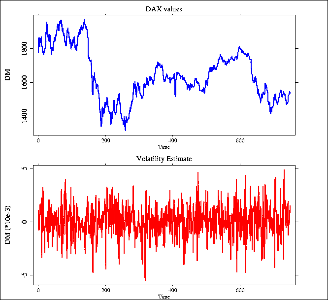
A volatility estimate of the DAX values (1990-1992)

The Finance library (``finance'')

In the last decades, there has been growing interest in the behaviour of financial markets. Due to the increasing globalisation of markets, they began to play a central role in international business and economic decision making. Thus the meaning of ``risk'' became the central theme in this context. Two approaches to deal with risk are prediction of financial time series and the so called ``hedging strategies''.

Investors, who want to avoid the risk of their long positions in financial assets could try to hedge the risk by going short in options on that asset and adapting the proportion held in assets and short-selled options according to the underlying price process of the asset. Therefore formulas for the pricing of derivative securities generated a lot of practical and theoretical interest.

Already in the year 1900, Bachelier introduced Brownian motion as a model for price fluctuations on a speculative market. In 1973 Black and Scholes found a formula for calculating the fair price (i.e. the absence of arbitrage possibilities) of an option.

In recent years, option pricing by discrete time series models, where the volatility process follows an ARCH or GARCH model have become more popular.

Details

The library ``finance'' contains macros for the evaluation of general price fluctuation processes. As a canonical mathematical model for these processes

is taken, where r is a parameter for the trend of the process, is the volatility process and is Brownian motion.

It contains menus for changing parameters and generating different time series scenarios. The actual values of assets as e.g. stock prices or exchange rates are computed by different methods. Prices of both European and American derivative securities are interactively determined analytically (Black/Scholes and McMillan) or numerically by a binomial tree.

The ``finance'' library provides different simulation tools for movements of assets driven by Brownian motion, GARCH and TGARCH processes, calculates actual fair prices of assets and their derivatives as the arbitrage from different portfolio and hedging strategies. Moreover, you can estimate and visualize the influence of different option price determining factors.

An Example

An important example is the investigation of different scenarios for the simulation of asset price fluctuations and and their impact on asset price structures. In XploRe, you can interactively change the parameters of the underlying price processes and visualize the effects on the prices in the different scenarios. In the following plots, asset prices were simulated by ARCH and GARCH processes. Depending on the moneyness (whether the security is in the money or not) of the option, the differences of Black/Scholes prices and those underlying the neutral risk pricing-method under ARCH and GARCH models were calculated and plotted.

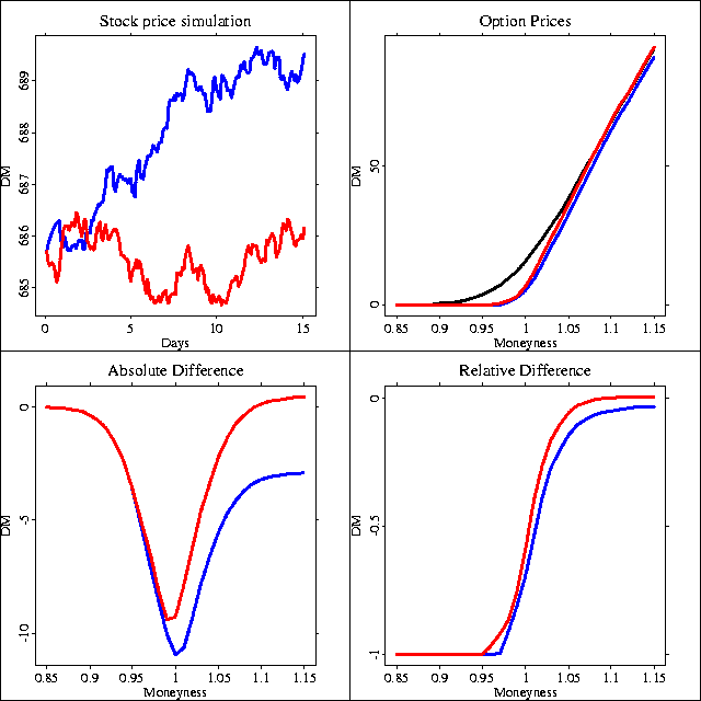
Differences between Black/Scholes, GARCH & TGARCH option prices

An Example

Another important tool for decision making in trading with derivatives is the analysis of the influence of different price determinig factors. Scenarios are used to determine the influence of a set of given factors. In XploRe, you have the possibility to estimate and simulate the influence of these factors on the security prices.

In the following graphic, you can see an example of these examining tools. It visualizes the influence of the exercise price and the volatility on option prices.

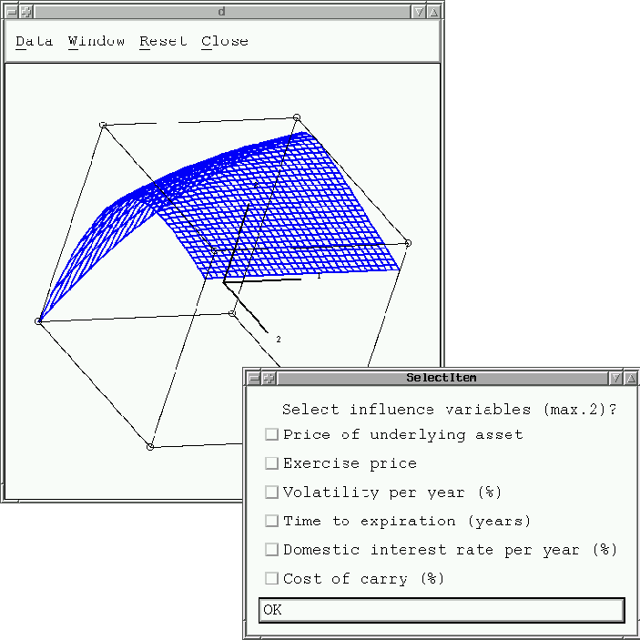
The influence of option price determining factors

The Micro-Econometrics library (``metrics'')

In economic applications one is often confronted with the phenomenon of limited dependent variables. This refers to censored or truncated regression models in which the range of the dependent variable is constrained in some way. These models are also called Tobit models. Next to their use in econometrics, these models are used in biometrics and engineering.

The recent increase in the availability of microeconomic sample survey data - i.e. datasets where the unit of analysis is e.g. an individual, a household or a firm - and the advance in computer technology, that has made estimation of large-scale Tobit models feasible, led to an increasing research on statistical methods to analyze such data. As the number of available methods grew, they have been subsumed under the heading microeconometrics.

Details

The library contains applications to those microeconometric problems. It contains several techniques for estimation of regression models from cross-section data with limited-dependent variables. You can estimate the classical Tobit model, as well as several recently developed variants. Moreover, methods are used that can be found in other XploRe libraries. Noteable examples include maximum likelihood estimators (see the library ``glm''), semiparametric estimators (library ``sim'') or discrete response models (library ``glm'').

The library offers several ways to estimate the parameters of a Type-II Tobit model, which is also commonly known as the self-selection model. It provides macros to estimate parametric (Heckman) and semiparametric versions of the self-selection model. Semiparametric estimation is possible in different ways. For example it can be based on kernel regression (Andrews, Powell) or the so called sliced inverse regression (SIR).

The Errors in Variables library (``eiv'')

Errors-in-variables models are concerned with the problem that independent variables can be measured with errors. This phenomenon takes often place in e.g. epidemiologic studies.

Ordinary errors-in-variables models are defined by

where one is unable to observe x directly. Instead of observing x you can only observe X. In addition, (x, e ,u) are generally normal distributed with mean (Mx,0,0) and covariance matrix . The observed variable X is sometimes called the manifest variable or the indicator variable. The unobserved variable x is called a latent variable in certain areas of application. u is often called measurement error. Thus, the above model is often called measurement error model. Models with fixed x are called functional models, while models with random x are called structural models.

Details

The macros in the library ``eiv'' focus mainly on normal distributed linear models. It contains estimation procedures like the method of moments for the etimation of the parameters of all types of models.

The Generalized Linear Models library (``glm'')

In many research fields (e.g. in biometrics or physics) one is confronted with data whose coherence is clearly non-linear. In these situations the classical linear regression approach is not appropriate. Moreover, in situations where the variable under examination is restricted e.g. to positive integers or a binomial value, the assumption of Gaussian error terms does not make much sense. The framework of Generalized Linear Models (GLM) summed up all the approaches that were formerly made to generalize the classical linear regression model.

Details

Generalized Linear Models (GLM) use a link function G to relate the mean of the response variable Y to the linear predictor :

where X are the predictor variables and the parameters of interest. The procedures implemented in XploRe refer to the monograph of McCullagh & Nelder.

The library ``glm'' enables to fit a variety of models, where the distribution of the output variable Y can be chosen out of various distribution types like Normal, Binomial, Poisson, Gamma, Inverse Gaussian, Geometric or Negative Binomial. The library provides comfortable interactive and non-interactive estimation routines for all these models. These models are estimated by Maximum-Likelihood-Estimation using either the Newton-Raphson or the Fisher scoring algorithm. The iterative estimation can be tuned interactively by several control options.

The routines in this library are able to handle special cases as prior weights, replications (automatic search for replications) and constraints on parameters (fix parameters). The output comprises a number of statistical characteristics of the estimated model like degrees of freedom, the deviance of the estimated model, the Pearson statistic, the log-likelihood of the estimated model, Akaike's AIC and Schwarz' BIC criterion, the (pseudo) coefficient of determination and its adjusted version, the number of iterations needed, the number of replicated observations needed and more. These results can be passed to an output display. Moreover, statistical evaluation and model selection tools are available.

An Example

The lizard data (McCullagh & Nelder) reflect site preferences of two species of lizards. These site preferences are supposed to be dependent on height, diameter of the perch, whether the perch was sunny or shaded and the daytime (early, mid-day, late). The output variable in this example is binomialy distributed and thus leads to a so called binary choice model. Here, the index would be . With the logistic link function this yields a classical logit model.

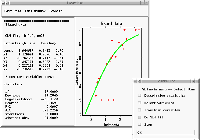
Estimation of the lizard data in the library ``glm''

The Generalized Partial Linear Models library (``gplm'')

In many application fields, it has turned out, that the assumption that the predictor is a linear function in X is too restrictive. Therefore nonparametric methods have been imposed in the GLM approach. This canonically led to a class of extensions of Generalized Linear Models, the so called Generalized Partial Linear Models (GPLM) which builds a semiparametric generalization of GLM.

Details

In Generalized Partial Linear Models (GPLM) a part of the predictor is allowed to be estimated in a nonparametric way. This means, the mean of the response variable Y can be expressed as

where X are predictor variables to be included linearly via a parameter and T predictor variables to be included via a nonparametric function .

The library (``gplm'') enables to fit all the models also available in ``glm''. The distribution of the output variable Y can be chosen out of various distribution types like Normal, Binomial, Poisson, Gamma, Inverse Gaussian, Geometric or Negative Binomial. As the ``glm'' library, it provides comfortable interactive and non-interactive estimation routines for all these models. These models are estimated by Maximum-Likelihood-Estimation using either the Newton-Raphson or the Fisher scoring algorithm. The iterative estimation can be tuned interactively by several control options.

As the ``glm'' library, this library is designed to handle the special cases as prior weights, replications (automatic search for replications) and constraints on parameters (fix parameters). Accordingly, the output comprises a number of statistical characteristics of the estimated model like degrees of freedom, the deviance of the estimated model, the Pearson statistic, the log-likelihood of the estimated model, Akaike's AIC and Schwarz' BIC criterion, the (pseudo) coefficient of determination and its adjusted version, the number of iterations and of replicated observations needed etc. These results can be passed to an output display. Moreover, statistical evaluation and model selection tools are available.

An Example

Credit scoring is a typical example for the use of GLM and GPLM. Suppose a credit institute is studying the payment behaviour of its clients. As input, variables like age of the client or total amount of credit can be viewed. The only information of interest in this case could be whether a given client is a ``good'' or a ``bad'' one. This output variable is binomialy distributed and this leads to a binary choice model. Here, the risk index would be with the logistic link function . This yields to a classical logit model. In the following graphic, the performance curve is a visualization of the missclassification rate. The figure compares the missclassification rates of a parametric GLM and a semiparametric GPLM fit.

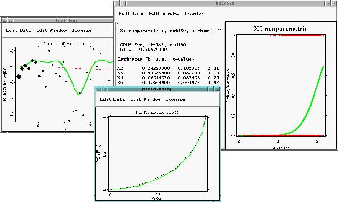
Credit scoring

The Generalized Additive Models library (``gam'')

In the estimation of multidimensional regression models, usual nonparametric methods without any restrictions, need an enormous number of observations to achieve a reasonable estimate of the multidimensional regression function. This is the so called ``curse of dimensionality''. Another problem would be the interpretability since you can not visualize or get an image of functions with more than two dimensions.

It is well known that you can get around the curse of dimensionality by restricting the regression problem to an addtitive model. Further these kind of models are easy to interpret. The additive components describe the influence of each variable separately.

Details

Additive regression models are defined by

where Y is the response and X the explanatory variable, are arbitrary unknown smooth functions and c a constant.

There exist mainly three ways to estimate this model: backfitting, based on a orthogonal function basis or on the integration estimator. The latter one estimates marginal influences of the for almost any kind of model. In an additive model their sum is the regression. The other procedures are looking in the space of additive models for the optimal fit for the given regression problem.

Natural extensions of the additive model are partial linear models, which include a linear part and generalized additive models which take the form

with a known link function G.

All the methods mentioned above to estimate in additive models, partial linear additive models or generalized versions with link function (logit, probit and others) can be done interactively in the ``gam'' library. This includes the backfitting and different kinds of integration methods. Moreover, regressions on principal components can be calculated as well as on the first and second derivatives of the additive components. This is important e.g. in economics for the estimation of elasticities or returns to scale.

Further the library ``gam'' contains test procedures for additive component analysis, like testing significance or linearity.

An Example

Generalized additive models are often used in the context of highly nonlinear phenomena as they occur e.g. in estimating production or consumption functions.

As an example consider a partially linear additive model

where is a sine, a quadratic function and Z a matrix of linear influence factors like discrete regressors, intercept and dummy variables etc. , and are estimated nonparametrically together with their first derivatives. The derivatives could be interpreted as the corresponding nonconstant elasticities.

In the following graphic you can see the estimated values for beta in the XploRe output window as well as the plots of the true and the estimated additive functions.

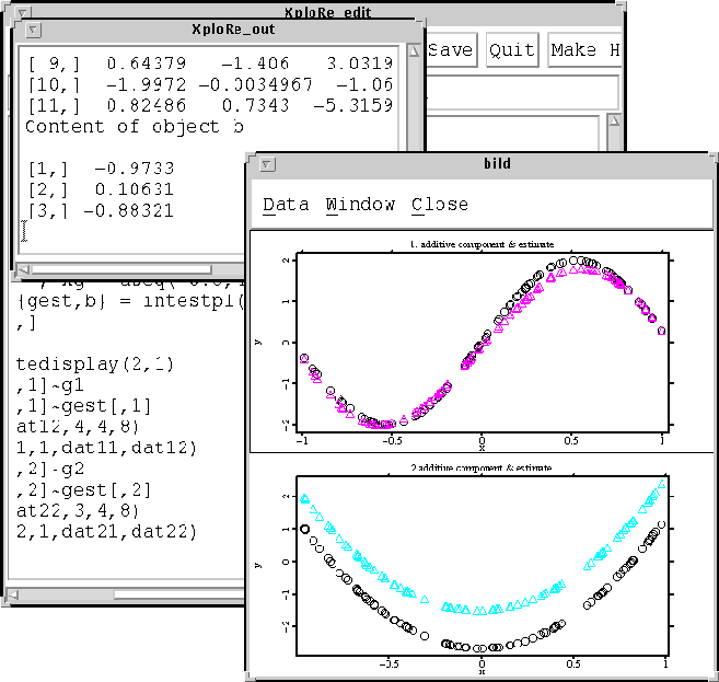
True vs. estimated function

The Single Index Models library (``sim'')

Another possibility to get around the problems concerning the interpretability and the curse of dimensionality in estimating multidimensional regression models while using nonparametric methods, are Single Index Models (SIM).

Well known in the world of parametric estimation are the GLMs. Unfortunately they restrict the model in the index to be linear and also the link function to be known. An extension to make these models more flexible is e.g. to allow for arbitrary link functions. This approach leads to single index models. They have the advantage to be easy interpretable since the coefficients in the index are simply the weights of the influence of each variable.

These kinds of models are e.g. used in economics (labour supply, migration, production functions).

Details

The library ``sim'' estimates regression functions with unknown links and linear index. It is mainly divided into three subjects; the first one is the estimation in pure single index models as a special kind of extension of the well known GLMs. The model is defined by

where G is the so called Link Function. The library provides estimation techniques as the the iterative optimization of a pseudo likelihood function. This proceeding is based on the work of Klein and Spady. Moreover, alternative methods like a direct estimator -- as the average derivative estimator (ADE) by Stoker -- are present in this library.

An additional task in the ``sim'' library is the possibility of testing against model specification with the aid of non- and semiparametric methods.

In contrast to the name of the library it not only provides single index models but also a possible extension. This is the possibility of calculating sliced inverse regression. In the ``sim'' library, the regression matrix for a projection on a k-dimensional index can be estimated.

An Example

Single index models are very often used in the context of credit scoring. Contrary to the use in GLM or GPLM it is not necessary to give an exact parametrization of the link function.

The following graphic demonstrates the power of single index models. Whereas the blue function is assumed to show the real coherence of the index and the varible of interest, the red function is their nonparametric estimate. You can see that even if the true function is known to you - what will not often be the case in applications to real data -, the results would not be much better in the parametrization case.

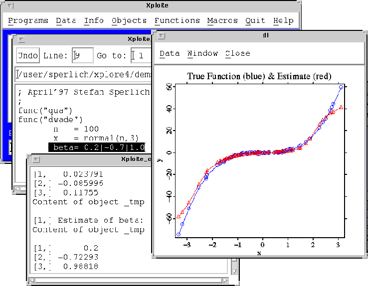
A true vs. an estimated link function

The Kernel Density and Regression library (``smoother'')

An important way of examining the overall structure (like e.g.\ symmetry, number and location of modes and valleys, and so on) of a given dataset is the use of nonparametric methods. Important graphical tools for understanding the association between a covariate and a response are nonparametric regression techniques. These techniques estimate the underlying regression function without any restrictive parametric form.

In most cases, nonparametric techniques are used as assistant tools for choosing the adequate parametric model by visually inspecting the estimated curve. Moreover, the nonparametric estimeates themselves describe the association between dependent and independent variables. The results can be used directly to understand and interpret the relationship between those variables.

Nonparametric smoothing provides powerful new tools for estimation of functions of unknown form, without the restraints of parametric models. Kernel based smoothing is easy to understand and has the advantage of good interpretability through the bandwidth, the width of windows used as local weight.

Details

The Kernel Density and Regression library of XploRe, so called ``smoother'' contains macros that implement many state-of-the-art methods for density estimation, regression, and derivative estimation. One distinguished feature of the ``smoother'' library is its interactive capability.

An estimate of an unknown density function f(x) is a weighted average of probability masses centered at each observation

where . The kernel K is a symmetric probability density and h>0 is the bandwidth.

In the theory of financial markets, models of the form,

are used to achieve nonparametric estimations of the diffusion processes of assets. To estimate the conditional mean function m(x), one solves a locally weighted least squares problem. This leads to the Nadaraya-Watson and the local linear estimators of m(x). Similarly, one can define other estimators and the corresponding local polynomial estimators of higher orders. All these estimates are available in higher dimensions as well in the smoother library.

The Kernel Estimation library

``kernel'' is a library which is needed to support the use of the tools providing nonparametric methods in XploRe It contains many commonly used kernel functions (like e.g. the Epanechnikov, the Gaussian or the Quartic kernel) and auxilliary functions. These kernel functions are used by several other routines which offer semi- and nonparametric procedures.

An Example

A good illustration of the functionalities of the ``smoother'' library is the macro bwsel, which does automatic bandwidth selection for density estimation. It gives the seven different options for the bandwidth selection (from the very old rule-of-thumb, to the sophisticated method of Sheather and Jones), and a new range of bandwidth for optimization when the initial search does not yield a solution.

A very famous example for a trimodal distribution is the chondrite data. It measures the percentage of silica in 22 chondrite meteors. The following graphic illustrates a univariate density estimation of this dataset. In that case the method Sheather & Jones plug-in was chosen from an interactive menu.

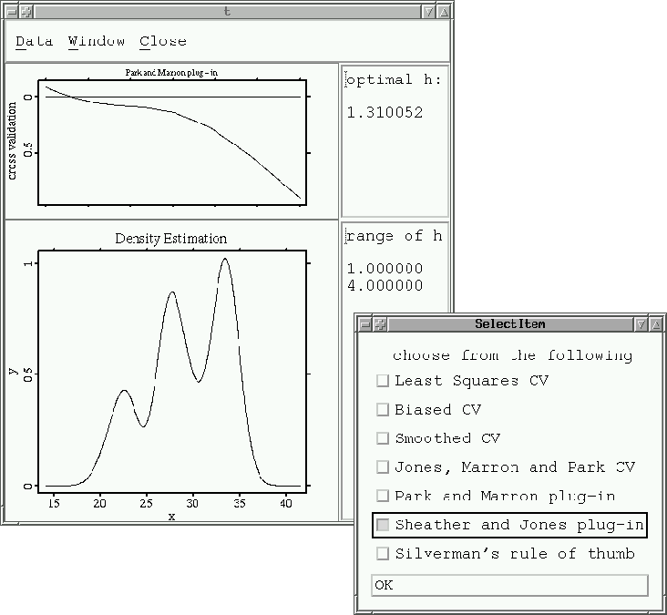
A univariate density estimation of the chondrite data

The Spline library (``spline'')

An alternative to fitting a classical linear regression model is the use of an additive model. This is a model of the form

with some arbitrary functions . A modern way to estimate such a model is the use of spline functions.

The smoothing splines method and the least squares splines method are two techniques of smoothing in statistics. The method of smoothing splines is much faster than the different kernel smoothing methods. Therefore, these method is very common in the backfitting of larger datasets.

Details

The library ``spline'' mainly inhabits these two methods. A smoothing spline minimizes a compromise between the fit and the degree of smoothness of the form

for n given pairs of observations and a smoothing parameter . This is a cubic spline with knots at the points . The parameters determining this spline are calculated by the algorithm of Reinsch.

You can calculate the cubic spline minimizing S(f) by choosing the smoothing parameter interactively. The parameter can be computed automatically by minimizing the cross-validation score by a Monte Carlo technique. Moreover, the splines can be calculated at any given set of nodes chosen by the user instead of the .

The method of least squares splines constructs an estimator that minimizes

for a given set of observations , where g denotes a cubic spline.

The space of polinomial splines of order 4 contains a basis of so called normalized B-splines. Therefore, the estimation problem reduces to the calculation of the normalized B-splines of order 4. The smoothing parameter corresponds with the number of nodes. The more nodes you have, the more the function is oscillating.

For a given dataset and given nodes, the least squares estimator and the corresponding normalized B-splines are calculated at the observations . Alternatively the user can choose any set of gridpoints to be taken instead.

An Example

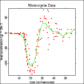
A common example for the illustration of nonparametric smoothing methods is the motorcycle data. The data consists of 133 observations of the time (in milliseconds) after a simulated impact with motorcycles and the head acceleration (in g) of a test object.

In the following graphic you can see the estimation of the least-squares spline at the nodes (16, 17, 30, 40) where the nodes were chosen by graphical inspection.

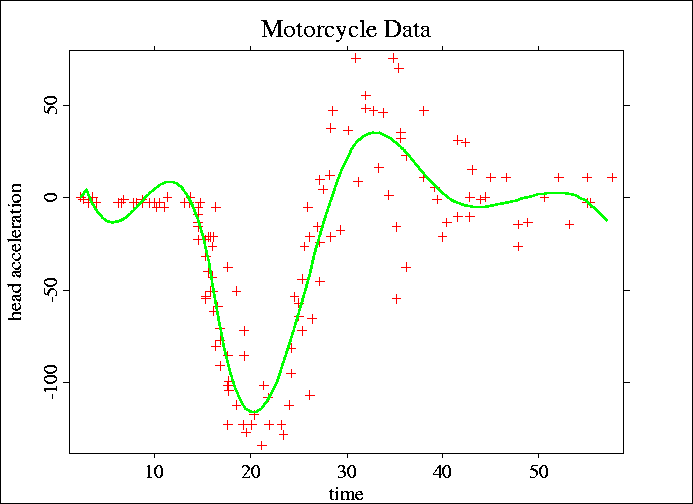
A spline regression on the base of normalized B-splines

The Neural Networks library (``nn'')

Neural Networks are a method for regression and classification of data. They construct a relation between given input and output units and provide an estimation of the functional form of this relation. The output of each unit is calculated by an activation function of its input. For better fitting results, a neural network can also contain hidden units. These are appropriate to model e.g. effects of unknown influence variables.

The strength of neural networks lies in their ability of learning, i.e., they can, so to say, be ``trained'' to fit, and their great flexibility. They provide an estimation of a qualitative expression about how input and output, or in general, your variables of interest and your variables of determination, are related. The most common tools in the context of neural networks are the feedforward neural networks which apply in computer science (e.g., computer learning), economics (e.g. credit scoring), molecular biology (e.g., protein structure prediction, prediction of functional sites at the DNA), and many other fields.

Details

The neural networks implemented in XploRe are multilayer feedforward neural networks with additional hidden layers. Mathematically, they can be written in the form



where is a nonlinear activation function and is typically either a linear or a sigmoidal activation function. represents the value of the k-th response variable given the k-th output unit.

Neural networks are fitted with an iterative optimization procedure which minimizes a given error function (e.g., the average mean squared error, the Kullback-Leibler distance) between the actual net output and a target output for the n-th object. This is the so called learning.

In the library ``nn'' a feedforward neural network can be fitted completly menu driven. You can interactively generate a multi layer feed forward network for a given dataset, train the network, run a crossvalidation over the decay parameter, change the parameters which are associated with the training process, choose the error function, choose the initialization of the weights, change between different graphical methods for visualizing the topology of the network and more. The visualization of your results can be chosen completly interactively and the results can be saved and restored later.

An Example

The swiss banknote data consists of 100 forged and 100 genuine banknotes. The input variables are width of the banknote, height of the left side of the banknote, height of the right side of the banknote, distance between the top of the inner box to the upper border, distance between the bottom of the inner box to the lower border and diagonal of the inner box. The aim is to find a classification rule to decide whether a new banknote is forged or genuine. The output unit contains a sigmoid activation function which means we are estimating . Thus we have to decide at which cut-off t we classify a banknote as forged (). In this example, XploRe by fitting a feedforward neural network.

The Wavelets library (``wavelet'')

A wavelet is, as the name suggests, a small wave. Many statistical phenomena have wavelet structure. Often small bursts of high frequency wavelets are followed by lower frequency waves or vice versa. The theory of wavelet reconstruction helps to localize and identify such accumulations of small waves and helps thus to better understand reasons for these phenomena. Wavelet theory is different from Fourier analysis and spectral theory since it is based on a local frequency representation.

The application of wavelet ideas to nonparametric statistics is relatively new and has drawn much attention by statisticians. Wavelets are also used in other fields like approximation theory, sound analysis and image compression. One of their basic properties is that they provide a sparse representation of smooth functions, even if the degree of smoothness varies considerably over the domain of interest or if the function is only piecewise smooth. These favorable approximation properties, which are not shared by the classical Fourier basis, lead to a superior performance of estimators of functions with spatially inhomogeneous smoothness properties compared to classical linear estimators.

Details

The library (``wavelet'') provides many smoothing routines and estimation procedures using wavelet techniques. You can generate Fast Wavelet Transforms (FWT) of multidimensional functions in either a multiresolution wavelet basis or a anisotropic wavelet basis. These methods are appropriate under both isotropic and anisotropic smoothness constraints.

Vice versa, a multidimensional function is derived from the wavelet coefficients in these bases as well as the mother and father wavelets. The translation invariant can be calculated with automatic hard thresholding or smoothed mother and father wavelets with the resulting estimates can be generated.

An example

The interest of financial market analysts is to understand reasons for inherent volatility and to find stochastic variance patterns. Below is shown a time series of log(ask) - log(bid) spreads of the DeutschMark (DEM) - USDollar (USD) exchange rates. The bid-ask spread varies dominantly between 2 - 3 levels, has asymmetric behavior with thin but high rare peaks to the top and more oscillations downwards. Wavelets provide a way to quantify this phenomenon and thereby help to detect mechanisms for these local bursts.

The plot shows the Bid - Ask spreads on the vertical axis. The horizontal axis denotes time for each quarter. The first part shows the wavelet estimator of the series and the second shows the size of wavelet coefficients that tell us the location and frequency of high frequency bursts.

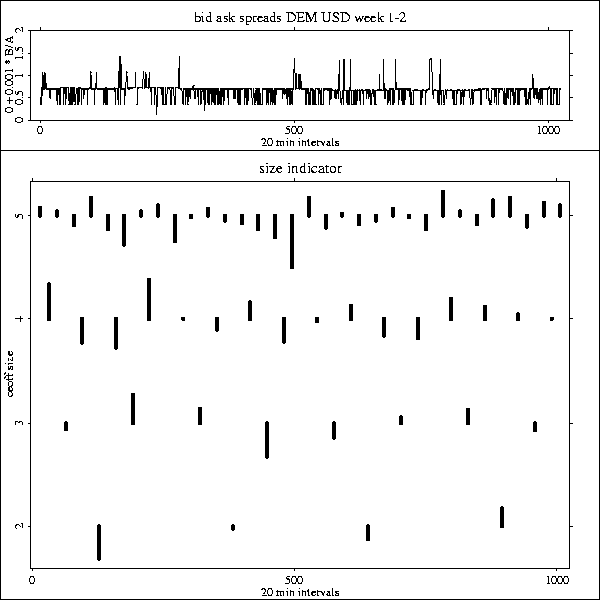
The wavelet estimation and the wavelet coefficients