Solutions to Practice Exam.

1. The first statement is True. This was stated in lecture.

The second statement is False. We expect about 68% of the data will be in the range $\bar{x} \pm s$. This was stated in lecture. See also pp. 64-65 in the text.

The third statement is False. A correlation of means there is no linear association between the variables. There may still be a nonlinear association.

The fourth statement is True. This was stated in lecture.

The fifth statement is False. The IQR will not be affected much whereas the standard deviation will be affected a lot. The IQR is a resisitant measure of spread (see pp. 40-42) whereas the sample variance is not (p. 49).

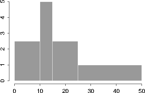
2. For a density histogram, the height of the bar is the relative frequency divided by the class interval width. The relevant calculations are shown below, and the plot follows.

Class 1c|Class Rel. 1c|Bar

Int. 1c|Int. Width Freq. 1c|Height

0 - 10 10 25% 2.5

10 - 15 5 25% 5.0

15 - 25 10 25% 2.5

25 - 50 25 25% 1.0

3. By calculator $\bar{x}$ = 8 and s = 3.74. If you got 3.24 for the standard deviation, your calculator is probably computing the ``wrong'' standard deviation by our definition.

4. Plot D is clearly a strong positive correlation, so it must correspond to (iv) r = +0.9. Plot B is a clear negative correlation which is fairly strong, so it must correspond to (iii) r = -0.8. Now we have to sort out plots A and C. Plot A seems to have a slight upward tilt, whereas if plot C has any tilt, it seems to be downward. So plot A goes with (ii) r = +0.4 and plot C with (i) r = 0.0.