Using S-Plus to do the work.

  Now we look to a much nicer stat package for the kinds of things we had to work our SAS off to get done in the previous section. In Splus, just type in commands in the X-window at the Splus prompt. Invoke Splus in unix with "Splus" at the unix prompt (or "/usr/site/splus-3.4/bin/Splus" if you want to use the old version):

long-eared% /net/owlnet-d/splus-3.4/sunos5/Splus
License Warning : S-PLUS license expires Sun Feb 28 23:59:59 1999
S-PLUS : Copyright (c) 1988, 1996 MathSoft, Inc.
S : Copyright AT&T.
Version 3.4 Release 1 for Sun SPARC, SunOS 5.3 : 1996 
Working data will be in /home/dcox/.Data 
> #LINES BEGINNING WITH # ARE MY COMMENTS
> #getting a nice help window to pop up:
> help.start()
> #setting up my graphics window
> X11()
> #reading in the data
> cow_scan("cow.dat")
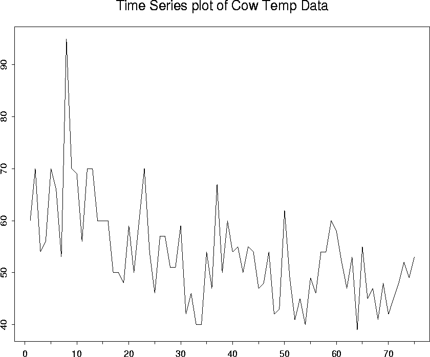
> #getting the time series plot
> tsplot(cow)
> title(main="Time Series plot of Cow Temp Data")
> #I clicked the print button in the graphics window 
> #you may have to pull down menu to get it.
> #the lagged scatterplot is pretty easy:
> length(cow)
[1] 75
> plot(cow[1:74],cow[2:75])
> title(main="lagged scatterplot of Cow Temp")
> #getting the sample autocorrelation:
> cow.acf_acf(cow)
> #how nice - the plot automatically appeared in my graphics window
> #(I knew that was going to happen because I had a help window on acf).
> #reading off the values of the sample acf
> cow.acf
$acf:

, , 1
            [,1] 
 [1,] 1.00000000
 [2,] 0.41050526
 [3,] 0.42295676
 [4,] 0.40500629
 [5,] 0.37264368
 [6,] 0.16299552
 [7,] 0.23204538
 [8,] 0.28196126
 [9,] 0.17605424
[10,] 0.03111671
[11,] 0.13753711
[12,] 0.05245340
[13,] 0.07643106
[14,] 0.09952299
[15,] 0.20836592
[16,] 0.20593612
[17,] 0.07179738
[18,] 0.07695194
[19,] 0.12802924

$lag:

, , 1
      [,1] 
 [1,]    0
 [2,]    1
 [3,]    2
 [4,]    3
 [5,]    4
 [6,]    5
 [7,]    6
 [8,]    7
 [9,]    8
[10,]    9
[11,]   10
[12,]   11
[13,]   12
[14,]   13
[15,]   14
[16,]   15
[17,]   16
[18,]   17
[19,]   18

$n.used:
[1] 75

$type:
[1] "correlation"

$series:
[1] "cow"
> #more than I really wanted, but I see the acf at lags 1 and 2 are
> #0.41050526 and 0.42295676
> #that's all for now
> q()

When the session is over, there were three new files in the working directory: ps.out.0001.ps, ps.out.0002.ps, and ps.out.0003.ps. These are postscript files which are shown below.

  

Figure 1: First plot.

  

Figure 2: Second plot.

  

Figure 3: Third plot.