Solution to Exercise 3.6.

Problem Statement: For the AR(2) process

$$Z_t - Z_{t-1} + 0.5 Z_{t-2} \; = \; a_t ,$$

(a) Calculate $\rho_1$.

(b) Using $\rho_0$ and $\rho_1$ as starting values and the difference equation form for the ACF, calculate the values of $\rho_k$ for $2 \le k \le 15$.

(c) Use the plotted function to estimate the period and damping factor for the ACF.

(d) Check the values in (c) by direct calculation using the values of $\phi_1$ and $\phi_2$.

Solution: First of all, let's check for stationarity. I know that wasn't explicitly stated to do, but the rest of the problem doesn't make sense without it. So we find the roots for

$$1 - w + .5 w^2 \; = \; 0 ,$$

which are

$$w_{\pm} \; = \; \frac{1 \pm \sqrt{1 - 4*(.5)}}{2*.5} \; = \; 1 \pm i ,$$

which are complex conjugate roots of modulus $\sqrt{2} \gt 1$, outside the unit circle.

OK, now to part (a). By (3.2.27), p. 62,

$$\rho_1 \; = \; \frac{\phi_1}{1-\phi_2} \; = \; \frac{1}{1-(-.5)} \; = \; 2/3 .$$

For part (b), the difference equation from (3.2.19), p. 60 is

$$\rho_k \; = \; \phi_1 \rho_{k-1} + \phi_2 \rho_{k-2} \; = \; \rho_{k-1} - .5 \rho_{k-2} , \quad k \gt 0 .$$

So, for instance,

Of course, you may not have had so much patience computing all those fractions. It's easy enough to write a little program to do it. Here is my Splus program, which I wrote to generate the plots on the AR(2) web page (here). Anyway, I also wrote some Matlab code toddo it:

» phi1=1;
» phi2=-.5;
» rho=[1 2/3 ];
» for k=2:15
rhok=phi1*rho(k)+phi2*rho(k-1);
rho=[rho rhok];
end
» plot(0:15,rho,'o')
» hold on
» plot([0 15] , [0 0], 'r')
» for i=0:15
plot([i i],[0 rho(i+1)])
end
» xlabel('Lag')
» ylabel('rho')
» title('Plot of ACF for Ex. 3.6')

The plot is shown below.

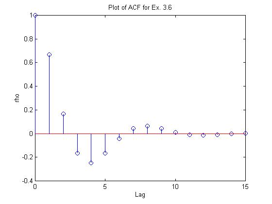
From this I would estimate the period at 8. The first time the ACF is negative is at lag 3, then positive at lag 7, then negative again at lag 11 (8 units after lag 3). For the damping factor, let's look at the peak values (where the damped cosine wave has a cosine factor of about 1). We see at lag 4 a negative peak of -1/4, then at lag 8 a positive peak of 1/16, then at lag 12 a negative peak of -1/64. So, it looks like $\rho_k$ is damped by a factor of 1/4 in 4 lags, so the damping factor should be about (1/4)^1/4 = $1/\sqrt{2}$.

OK, let's see how it squares with the computation. We know the ACF is of the form

$$\rho_k \; = \; A_1 G_1^k \, + \, A_2 G_2^k ,$$

where G_i^-1 are the roots of the characteristic polynomial and the A_i are coefficients determined from initial conditions (see e.g. (3.2.20), p. 60). In this case, we already know they are complex conjugate roots, so (3.2.21), p. 60 applies and we can write the ACF in the form

$$\rho_k \; = \; D^k \sin ( 2 \pi f_0 k + F) / \sin F ,$$

where D is the damping factor, f₀ the frequency, and F the phase. Here,

$$D \; = \; \vert G_i \vert \; = \; 1/\vert 1 \pm i \vert \; = \; 1/\sqrt{2} ,$$

and

$$2 \pi f_0 \; = \; \mbox{Arg } G_+ \; = \; \arg{1 + i} \; = \; \pi/4 ,$$

since the angle between 1+i and the real axis is 45^o, so

$$f_0 \; = \; 1/8 ,$$

and the period is 1/f₀ = 8. Note that these match exactly with my ``guesses'' above.