Solution to Exercise 3.7.

Problem Statement: (a) Plot the power spectrum g(f) of the AR process in Exercise 3.6 and show that it has a peak at a period which is close to the period in the ACF.

(b) Graphically or otherwise estimate the proportion of the variance of the series in the frequency band between f = 0.0 and f = 0.2 cycle per data interval.

Solution: The spectrum p(f) for a general AR(2) process is given in (3.2.29), p. 63. The power spectrum is g(f) = $p(f)/\sigma_Z^2$. See (2.2.13), p. 40. From (3.2.28), p. 62 we have $\sigma_a^2/\sigma_Z^2$ = $1-\rho_1 \phi_1 - \rho_2 \phi_2$ = 1 - 2/3 + 1/12 = 5/12. For our case:

The plot is shown below.

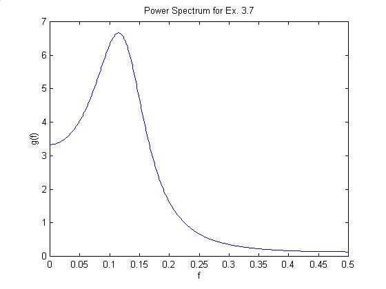
The maximum is pretty close to f = 1/8 = .125. It's actually about .1150 from numerical minimization (fmin in Matlab).

I'm not sure the point of part (b), but it's clear that most of the area is in the range of to .2. Anyway, numerical integration using the Matlab quad function gives .8853 out of a total area of 1 (I would have guessed about 90% from looking at the graph).

Just for fun, I've given a plot of a realization of such a process below.

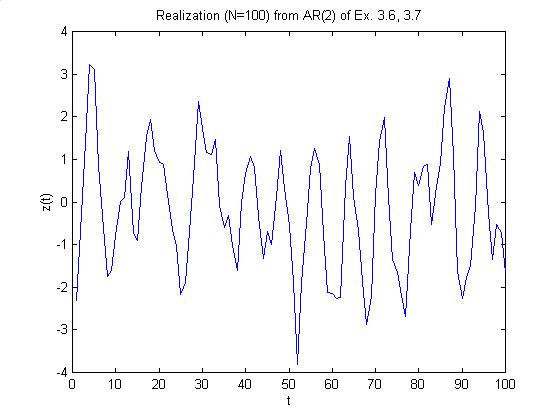
Note that it looks quasiperiodic and has about 12 periods in the record of 100 observations (as would be predicted from a period of 8).