Suppose X is a r.v. (random variable) with density
![]() . If its distribution is discrete, then
the density is also known as the probability mass
function and in fact gives the ``point'' probabilities:
. If its distribution is discrete, then
the density is also known as the probability mass
function and in fact gives the ``point'' probabilities:
![]()
Probabilities of sets with multiple points are obtained by summing:
![]()
If the distribution of X is continuous, then all point probabilities are 0 and the density gives probabilities of intervals through integration:
![]()
For The mathematical expectation of a function of a r.v. is defined to be

The formulae displayed here illustrate the
general principle: summations for discrete r.v.'s
and integration for continuous r.v.'s. Also,
whenever the limits of integration or summation
are not shown, it is assumed that they are over
the entire ``space,'' which effectively means
all values of x where ![]() .
.
Technical Note:
To define E[h(X)], it is usually required that either
(i) ![]() so that the summands or integrand is never
negative, and then E[h(X)] may possibly be
so that the summands or integrand is never
negative, and then E[h(X)] may possibly be ![]() , or
(ii)
, or
(ii) ![]() , which means effectively
that the summation or integration converges absolutely.
We will generally not bother ourselves with such details.
We always asssume that the integral or summation satisfies
whatever mathematical properties are needed for things to
make sense. There are very few practical situations where
problems of infinite expectation arise.
, which means effectively
that the summation or integration converges absolutely.
We will generally not bother ourselves with such details.
We always asssume that the integral or summation satisfies
whatever mathematical properties are needed for things to
make sense. There are very few practical situations where
problems of infinite expectation arise.
The connection between mathematical expectation and data
comes through the notion of long run averages:
If ![]() ,
, ![]() ,
, ![]() ,
, ![]() is a sample of realized
values of the r.v. X, then as
is a sample of realized
values of the r.v. X, then as ![]() the sample mean
the sample mean ![]() tends to
E[h(X)]. The precise mathematical formulation of
this ``principle'' is the Law of Large Numbers, which
makes certain assumptions on how the sample is generated
(e.g. that the sample are realized values of independent
and identically distributed (abbreviated i.i.d.) random
variables with the same distribution as X).
tends to
E[h(X)]. The precise mathematical formulation of
this ``principle'' is the Law of Large Numbers, which
makes certain assumptions on how the sample is generated
(e.g. that the sample are realized values of independent
and identically distributed (abbreviated i.i.d.) random
variables with the same distribution as X).
Of course, there are certain mathematical expectations which are of most interest, namely the mean and variance of the r.v.:

Some useful properties of these mathematical ``operators'' are summarized in the next proposition. Note that if X and Y are r.v.'s, then so are h(X) and g(X,Y) for any appropriately defined real valued functions h(x) and g(x,y).
Proof. Part (i) is proved in Hogg & Craig. For part (ii), assuming X is a continuous r.v. we have

For (iii) we apply the version of Chebyshev's inequality that
says if X is a nonnegative r.v. and c > 0 then
P[X > c] ![]() E[X]/c. See Hogg & Craig. Since
E[X] = 0, it follows that P[X > c] = 0 for all
c > 0. In particular, P[X > 0] =
E[X]/c. See Hogg & Craig. Since
E[X] = 0, it follows that P[X > c] = 0 for all
c > 0. In particular, P[X > 0] =
![]()
![]()
![]() = 0. Since we
know
= 0. Since we
know ![]() we have 1 =
we have 1 = ![]() =
P[X = 0] + P[X > 0] = P[X=0].
=
P[X = 0] + P[X > 0] = P[X=0].
![]()
Proof.
Since the r.v. ![]() is nonnegative, it follows
that
is nonnegative, it follows
that ![]() =
= ![]()
![]() 0 by part (ii)
of Proposition 1. Continuing with the fact that
0 by part (ii)
of Proposition 1. Continuing with the fact that
![]()
![]() 0, if 0 =t
0, if 0 =t ![]() =
= ![]() ,
then by part (iii) of Proposition 1 it follows that
the r.v.
,
then by part (iii) of Proposition 1 it follows that
the r.v. ![]() = 0 with probability 1, i.e.\
= 0 with probability 1, i.e.\
![]() with probability 1. Since
with probability 1. Since ![]() is a constant,
the completes the proof of part (i) of Proposition 2.
is a constant,
the completes the proof of part (i) of Proposition 2.
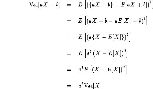
For part (ii), note from part (i) of Proposition 1 that E[a X + b] = a E[X] + b, so

Part (iii) is already proved in Hogg & Craig, right after
the definition of variance.
![]()
The corresponding ``sample'' quantities are given by
An ``alternative'' sample variance is sometimes considered::
The difference between the two sample variances is unimportant when n is large.