An Example of Asymptotics: Confidence Intervals for a Binomial p Based on Normal Approximation.

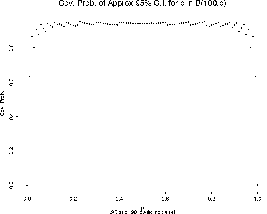
Here, we compute the actual coverage probability of the ``usual'' confidence interval for the success probability p in a Binomial Experiment. This interval is based on the normal approximation. Suppose where is unknown. If n is large (and p is not too close to 0 or 1), then the point estimate = Y/n has approximately a normal distribution. More precisely, is approximately N(0,1), or we say

 

Thus,

One can also show that

 

This will follow from Slutsky's theorem, and will be shown later in the course. Now with a little algebra on the inequalities defining the event we have

 

Thus,

 

gives an approximate confidence interval for p if n is large (and p is not too close to 0 or 1).

So the nominal coverage probability is , but what is the actual coverage probability? To investigate this, we wrote an Splus function to determine first what the confidence interval is for given values of n, y (the realization of Y), and the nominal coverage probability:

> Na0int
function(n, y, nominal)
{
# computes approx. confidence interval for binomial p
#   based on simple normal approx. with given "nominal" cov. prob.
#
        alpha <- 1 - nominal
        zalpha <- qnorm(1 - alpha/2)
        phat <- y/n
        se <- sqrt((phat * (1 - phat))/n)
        halfwidth <- zalpha * se
        pmin <- phat - halfwidth
        pmax <- phat + halfwidth
        return(pmin, pmax)
}

Then we wrote an Splus function to compute the actual coverage probability for given p:

> Na0covprob
function(n, p, nominal)
{
# computes true cov prob of approx. confidence interval for binomial p
#   based on simple normal approx. with given "nominal" cov. prob.
#
        covprob.o <- 0
        covprob.c <- 0
        for(y in 0:n) {
                interval <- Na0int(n, y, nominal)
                if(interval[[1]] < p & p < interval[[2]])
                        covprob.o <- covprob.o + dbinom(y, n, p)
                if(interval[[1]] <= p & p <= interval[[2]])
                        covprob.c <- covprob.c + dbinom(y, n, p)
        }
        return(covprob.o, covprob.c)
}

We looped over the last one with n = 100, nominal coverage of , and for p = 0, 0.01, 0.02, , 0.99, 1.00. The results are plotted in Figures and . One sees that the actual coverage probability is above 0.90 for 0.09 < p < 0.91, and above 0.93 for 0.22 < p < 0.78.

  
Figure: Plot of coverage probability for nominal 95% confidence interval of p from B(100,p) observation based on normal approximation to binomial.

  
Figure: Plot of coverage probability for nominal 95% confidence interval of p from B(100,p) observation based on normal approximation to binomial for a smaller range of values of p.