Now consider a pair of r.v.'s (X,Y) with joint
density ![]() which may be either continuous
or discrete (or a mixture of discrete and continuous).
As we shall deal almost exclusively with continuous
random variables in time series applications, we will
implicitly assume that r.v.'s are continuous, but
the corresponding formulae for discrete r.v.'s can
be obtained by replace sums by integrals.
The covariance between X and Y (or
the covariance of X and Y; the appropriate
preposition is not entirely fixed) is defined to be
which may be either continuous
or discrete (or a mixture of discrete and continuous).
As we shall deal almost exclusively with continuous
random variables in time series applications, we will
implicitly assume that r.v.'s are continuous, but
the corresponding formulae for discrete r.v.'s can
be obtained by replace sums by integrals.
The covariance between X and Y (or
the covariance of X and Y; the appropriate
preposition is not entirely fixed) is defined to be
![]()
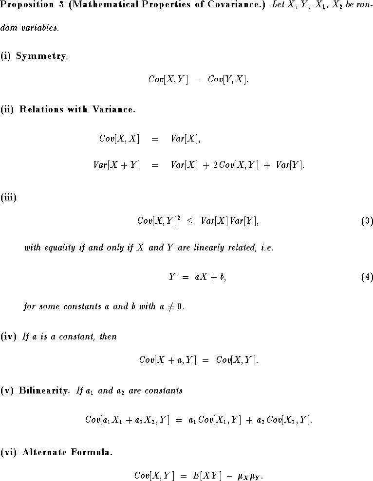
Useful facts are collected in the next result.
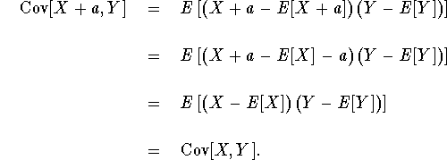
Proof. Part (i) is easy:
![]()
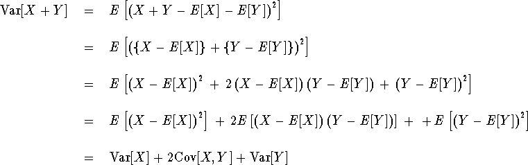
The first equation in part (ii) is trivial
(plug in Y = X in the definition ![]() .
For the second equation, one can find the result
in Hogg & Craig in the section on Expectations
of Functions of Random Variables, but it is not
explicitly stated, so
.
For the second equation, one can find the result
in Hogg & Craig in the section on Expectations
of Functions of Random Variables, but it is not
explicitly stated, so
Part (iii) is an exercise in Hogg & Craig, so we give its proof here, but after proving the remaining parts of the proposition. It is basically the Cauchy-Schwarz inequality in one guise.
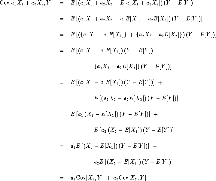
For part (iv), similarly to the proof of part (ii) of Proposition 2,
Part (v) is similar:
Part (vi) is already proved in Hogg & Craig.
Now we are ready to give the proof of part (iii). Let t be a real variable, then by (i) of Proposition 2,
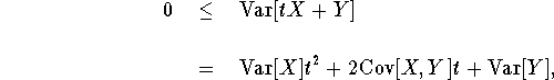
where the last equation follows by some ``algebra'' based on (ii), (v) above and (ii) of Proposition 2. Writing this in the form
![]()
we have a function of t this is a quadratic polynomial which is always nonnegative, so the discriminant is nonpositive, i.e.
![]()
from which it follows that
![]()
Now if we have equality, i.e.
![]()
then it follows that there is a value of t for which
Q(t) = 0, i.e. ![]() = 0 for some t,
and hence by (i) of Proposition 2,
tX + Y = c with probability 1
where C is a constant, and thus
Y = - tX + c which proves the claim.
= 0 for some t,
and hence by (i) of Proposition 2,
tX + Y = c with probability 1
where C is a constant, and thus
Y = - tX + c which proves the claim.
![]()
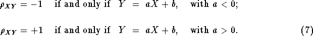
It follows from (i), (iv), and (v) of the last proposition that
The correlation or correlation coefficient is defined as
![]()
From part (iii), we have the Correlation Inequality:
and
From part (iii) of Proposition 3, we only
know that ![]() =
= ![]() implies
Y = aX + b with probability 1, but one can
check that a < 0 implies
implies
Y = aX + b with probability 1, but one can
check that a < 0 implies ![]() < 0
and similarly for a > 0.
We also have for any constants a, b, c, and d,
with a > 0 and c > 0,
< 0
and similarly for a > 0.
We also have for any constants a, b, c, and d,
with a > 0 and c > 0,
This follows by application of (iv) and (v) of Proposition 3 and part (ii) of Proposition 2.
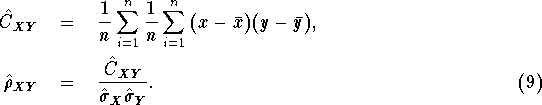
Given a sample of (X,Y) data, say
![]() ,
, ![]() ,
, ![]() ,
, ![]() ,
we can consider the sample covariance and correlation
defined by
,
we can consider the sample covariance and correlation
defined by
Of course, in the above ![]() and
and ![]() are
the sample mean and variance of the X sample
are
the sample mean and variance of the X sample
![]() ,
, ![]() ,
, ![]() ,
, ![]() , and
, and
![]() and
and ![]() are
the sample mean and variance of the Y sample
are
the sample mean and variance of the Y sample
![]() ,
, ![]() ,
, ![]() ,
, ![]() .
Note that we use the form (2) of the sample
variance here, although this is not entirely standardized.
.
Note that we use the form (2) of the sample
variance here, although this is not entirely standardized.