


Next: Solution to Exercise 6.12.
Up: No Title
Previous: Solution to Exercise 5.54.
Unfortunately, the data for this problem is not on the CD in the
back of the book. If I had realized that, I wouldn't have assigned
it. I will have to check for that in the future.
(a)
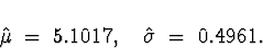
Anyway, after inputting the data into minitab, I took
logarithms and then got the mean and standard deviation of
those. The parameter estimates are
(b)
According to the formula on p. 181,
![\begin{displaymath}
E[X] \; = \; \exp[ \mu + \sigma^2/2 ] .\end{displaymath}](img27.gif)
Thus, our estimate of E[X] is
![\begin{displaymath}
\exp[ 5.1017 + (0.4961^2)/2 ]
\; = \;
185.8161\end{displaymath}](img28.gif)
Interestingly, the sample mean (of the raw
stream flow - not taking logarithms) is
185.4, which is almost exactly the same.
In this case, one can show mathematically
that the estimate based on the  and the
  above is in fact
more accurate than the sample mean as an
estimate of the ``population'' mean
E[X], provided the random sample
from the log-normal model is correct.
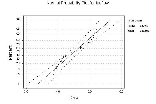
A normal probability plot of the logarithm
of flow is shown below.
above is in fact
more accurate than the sample mean as an
estimate of the ``population'' mean
E[X], provided the random sample
from the log-normal model is correct.
A normal probability plot of the logarithm
of flow is shown below.
Dennis Cox
3/22/2001